

Geophysical phenomena — from groundwater flow to seismic wave propagation — are governed by partial differential equations that describe how physical quantities change across space and time. Post 242 introduced the broader PDE framework for earth systems modeling, covering finite volume methods and the tools available for tackling these equations at scale. This article drills down into two practical domains where Python has transformed geophysical workflows: groundwater flow modeling and seismic wave modeling.
In both domains, Python has shifted the paradigm from proprietary, black-box software to transparent, reproducible research. Whether you’re setting up a MODFLOW groundwater simulation with FloPy or implementing a finite-difference wave equation solver with Devito, Python provides the same combination of mathematical clarity, ecosystem flexibility, and community support that has reshaped scientific computing across disciplines.
We’ll walk through concrete Python code examples, compare tool ecosystems (MODFLOW/FloPy vs Devito/SWEEP), and show how to select the right tool for your specific geophysical problem.
Groundwater Flow Modeling with MODFLOW and FloPy
Groundwater flow through porous media is one of the most mature applications of computational geophysics. The governing equations combine Darcy’s law with mass conservation, yielding a diffusion-type PDE that, despite its relative simplicity compared to seismic wave propagation, presents practical challenges in parameterization, boundary conditions, and numerical stability.
The Governing Equation
Groundwater flow follows Darcy’s law combined with mass conservation, producing the diffusion-type PDE:
∂∂x(Kxx∂h∂x)+∂∂y(Kyy∂h∂y)+∂∂z(Kzz∂h∂z)+W=Ss∂h∂t
\frac{\partial}{\partial x}\left(K_{xx}\frac{\partial h}{\partial x}\right) + \frac{\partial}{\partial y}\left(K_{yy}\frac{\partial h}{\partial y}\right) + \frac{\partial}{\partial z}\left(K_{zz}\frac{\partial h}{\partial z}\right) + W = S_s\frac{\partial h}{\partial t}
where
hh
is hydraulic head,
KK
is hydraulic conductivity,
WW
represents sources and sinks (wells, recharge), and
SsS_s
is specific storage [1].
The finite-difference discretization underlying MODFLOW is well-suited for structured grids, making it the industry standard for regional groundwater studies. But working directly with MODFLOW’s input files is tedious — that’s where FloPy enters.
Getting Started with FloPy
FloPy is a Python package that automates MODFLOW 6 workflows: it generates input files, runs simulations, and parses output for visualization. The ecosystem has expanded beyond FloPy itself to include modflow-setup (USGS, 2022) for workflow automation, SFRmaker for surface water-routing, and Linesink-Maker for streamflow routing. Together, they form a comprehensive ecosystem for groundwater model construction and automation [2].
Here’s a practical FloPy quick-start for a simple groundwater model:
import flopy
import numpy as np

# Define model parameters
model_name = 'simple_groundwater'
top = 100.0 # model top elevation
botm = 0.0 # bottom elevation
nlay = 10 # number of layers
nrow = 50 # number of rows
ncol = 50 # number of columns

# Create model simulation
sim = flopy.mf6.MFSimulation(sim_name=model_name, exe_name='mf6')
ibs = flopy.mf6.ModIbs(sim)
sts = flopy.mf6.ModSts(sim)

# Create model domain (discharge package)
dis = flopy.mf6.MFDischarge(sim, print_flows=True, save_first=True)

# Set up numerical grid
grid = flopy.mf6.MFModelGrid((nlay, nrow, ncol), top=top)

# Define hydraulic properties
k = np.full((nlay, nrow, ncol), 1e-3) # hydraulic conductivity (m/s)
hsy = np.full((nrow, ncol), 95.0) # head at surface (head boundary)
ss = np.full((nlay, nrow, ncol), 1e-4) # specific storage

# Create simulation and run
sim.create_simulation()
# ... set up stress packages, run simulation
The key advantage of FloPy is that it replaces dozens of MODFLOW input files with a single Python API. You define grid geometry, hydraulic properties, and boundary conditions as Python objects, and FloPy handles file generation, validation, and execution.
Visualization and Results
FloPy’s visualization capabilities make it straightforward to interpret simulation results. After running a simulation:
# Load model results
mf = flopy.modflow.Modflow(sim)
h = mf.hds.get_data()

# Plot head contours and flow vectors
model.plot_head()
model.plot_vector_flow()
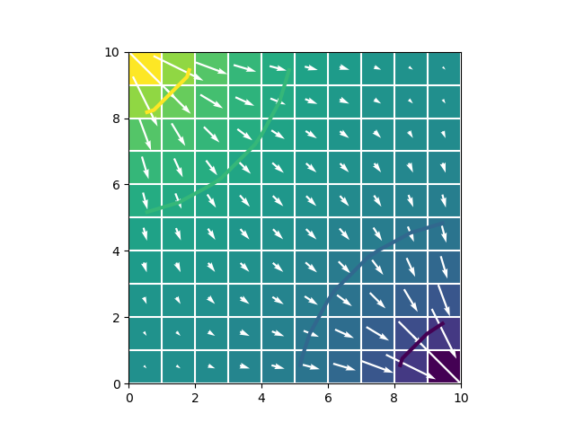
This produces head contour plots and vector flow visualization [3] — the kind of output that hydrogeologists use to interpret flow regimes, identify flow paths, and validate model behavior.
The visualization output from FloPy shows hydraulic head contours overlaid with flow vectors, making it easy to understand groundwater movement patterns in complex aquifer systems. The FloPy quickstart visualization demonstrates this capability clearly.
Attribution: FloPy quickstart.png — ModflowPy
Practical Workflow with modflow-setup
For larger projects, modflow-setup provides a YAML-based configuration approach that automatically constructs grids from source data. This represents the modern shift toward workflow automation — you define model structure in declarative configuration files, and modflow-setup handles the tedious geometry and property assignment.
The practical workflow looks like this:
- Define grid and aquifer properties (conductivity, storage coefficients, layer thicknesses)
- Set boundary conditions (constant heads, wells, recharge rates)
- Run simulation through FloPy’s automated MODFLOW 6 execution
- Visualize results with FloPy’s plotting utilities or export to Paraview for 3D rendering
For hydrogeologists working with regulatory groundwater models, this workflow is essential because MODFLOW remains the industry standard for applied groundwater regulation and management [4]. FloPy bridges the gap between research prototyping and production workflows — you get the reproducibility and flexibility of Python while maintaining regulatory acceptance of MODFLOW results.
Seismic Wave Modeling with Python
Seismic wave modeling is fundamentally different from groundwater flow. Where groundwater follows diffusion-type equations that smooth sharp features over time, seismic wave propagation follows the elastic wave equation — a second-order hyperbolic PDE that preserves sharp wavefronts and requires careful numerical treatment to avoid artificial dispersion.
The Wave Equation
The elastic wave equation governs seismic wave propagation:
∂2𝐮∂t2=∇⋅(𝐂:∇𝐮)+𝐟
\frac{\partial^2 \mathbf{u}}{\partial t^2} = \nabla \cdot (\mathbf{C} : \nabla \mathbf{u}) + \mathbf{f}
where
𝐮\mathbf{u}
is displacement,
𝐂\mathbf{C}
is the stiffness tensor, and
𝐟\mathbf{f}
represents body forces.
Unlike groundwater flow (where pressure diffuses and sharp gradients smooth), seismic waves propagate with minimal dispersion over thousands of kilometers — which means numerical schemes must preserve wavefront sharpness to produce accurate results. This makes finite-difference time-domain (FDTD) methods particularly attractive because they’re both efficient and accurate for wave propagation problems.
Devito: Symbolic DSL for Wave Equation Solvers
Devito (Georgia Tech SLIM Group) generates optimized C code for wave-equation finite-difference simulations using SymPy symbolic mathematics. The framework is designed for researchers who want differentiable wave propagation — essential for full-waveform inversion (FWI) and reverse-time migration (RTM) workflows.
Here’s the Devito TLE (Time-Lag Ensemble) forward modeling example from the SLIM tutorial:
from devito import Grid, TimeAxis, Function, TimeFunction
from devito import Eq, Operator, where
from scipy import sparse

# Define grid dimensions
nx, nz = 200, 200
space_order = 4
time_order = 2
time_steps = 100

# Create computational grid
grid = Grid(shape=(nx, nz))

# Define velocity model (m/s)
v = Function(name='velocity', grid=grid, data=1500.0 * np.ones((nx, nz)))

# Initialize wavefield
u = TimeFunction(name='u', grid=grid, time_order=time_order)

# Set up initial conditions
src = TimeFunction(name='source', grid=grid)

# Define wave equation operator
eq = Eq(u.forward, u.back + src + v**2 * u.laplacian)

# Create and run operator
op = Operator(eq)
op()

# Analyze results
import matplotlib.pyplot as plt
plt.imshow(u.data[-1].T, cmap='viridis')
plt.title('Wavefield snapshot')
plt.show()
This code demonstrates the key workflow: define a grid, specify a velocity model, set up the wave equation operator, and execute it. Devito’s SymPy-based symbolic engine translates the high-level equation into optimized C code that runs at near-native performance — a critical feature when simulating large seismic datasets.
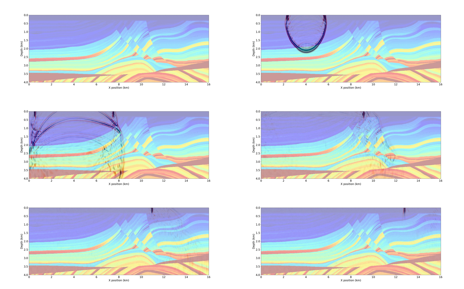
The SLIM group’s forward/backward wave propagation animation in the Marmousi model shows the kind of results Devito produces: clear wavefront propagation through a realistic velocity model [5]. This animation demonstrates both forward and backward wavefield evolution — the same wavefields that underpin FWI workflows.
Attribution: SLIM Forward.gif — SLIM group, Georgia Tech
SWEEP 2026: Automatic Differentiation for Seismic Inversion
The most significant recent development in Python seismic modeling is SWEEP, an arXiv paper published in April 2026 that introduces automatic differentiation as a primary alternative to manual adjoint-state derivations for seismic inversion. This represents a paradigm shift.
Traditional seismic inversion uses the adjoint-state method, where researchers manually derive adjoint equations and implement them as separate reverse-time propagation codes. SWEEP automates this process: by using automatic differentiation (AD) with native time-stepping schemes, practitioners can compute gradients directly from their forward model without deriving adjoint equations by hand.
SWEEP supports:
- Acoustic, elastic, and anisotropic wave equations (VTI, TTI)
- Automatic differentiation with JAX and PyTorch backends
- Multi-GPU batch modeling for large-scale inversion
- Unified wave equation framework that replaces separate forward/adjoint codes
The contrast with Devito is instructive: Devito uses symbolic DSL expressions where you write the wave equation as a symbolic formula and Devito generates optimized C code from it. SWEEP takes a different approach — you write native Python code for the forward model, and AD frameworks (JAX, PyTorch) compute gradients automatically through reverse-mode differentiation.
For practitioners, this means:
- Devito (symbolic DSL): Explicit, optimized C code; requires learning DSL syntax; gradients computed via symbolic adjoint generation
- SWEEP (automatic differentiation): Native Python code; gradients computed automatically by AD; flexible backends (JAX, PyTorch); potentially more intuitive for Python developers
Deepwave: GPU-Accelerated Adjoint-State Gradients
Deepwave (KIT Geophysical Institute) implements differentiable wave propagation in PyTorch, enabling GPU-accelerated full-waveform inversion and adjoint-state gradient computation. Unlike Devito’s symbolic approach, Deepwave works directly with PyTorch tensors and computes gradients through automatic differentiation — but requires explicit adjoint implementation rather than end-to-end AD.
Deepwave is particularly useful when you want GPU acceleration with PyTorch’s ecosystem, and you’re comfortable implementing adjoint-state methods explicitly.
Simwave: High-Performance Acoustic Wave Propagation
Simwave, published in 2025, fills a gap in the Python seismic ecosystem: high-performance acoustic wave propagation with verified C and GPU backends. It bridges the gap between research prototypes and production-grade geophysical tools — useful when you need performance that matches proprietary codes.
Practical Guidance: Choosing Your Tool
Selecting the right tool depends on your specific problem: domain, scale, and the role of your model in the research workflow. Here’s a practical comparison:
Tool Selection Guide
| Scenario | Recommended Tool | Strengths | When to Avoid |
|---|---|---|---|
| Regional groundwater flow | MODFLOW/FloPy | Industry standard; regulatory acceptance; large ecosystem | Custom multiphysics coupling (use FiPy instead) |
| Custom groundwater PDEs | FiPy | Flexible; supports coupled systems; Python-native | Regional regulatory modeling (use MODFLOW) |
| Seismic forward modeling (FWI-ready) | Devito | Differentiable; optimized C code generation; SLIM ecosystem | If you need automatic differentiation out-of-the-box (use SWEEP) |
| Seismic inversion with AD | SWEEP | Automatic differentiation; no manual adjoint needed; multi-GPU | If you’re locked into PyTorch only (consider Deepwave) |
| GPU-accelerated PyTorch workflows | Deepwave | Native PyTorch; GPU acceleration; KIT validation | If you need automatic gradient computation without manual adjoint (use SWEEP) |
| Production-grade acoustic modeling | Simwave | Verified C/GPU backends; high performance | Research prototyping (Devito or SWEEP may be more flexible) |
Best Practices for Geophysical Modeling
Whether you’re modeling groundwater or seismic waves, these practical guidelines apply across both domains:
- Start with analytical benchmarks: Before running complex models, verify your implementation against known analytical solutions. MODFLOW’s published benchmark problems and Devito’s tutorial notebooks provide this foundation.
- Pay attention to the CFL condition: In explicit seismic time-stepping, the time step must satisfy
Δt≤Δx2vmax\Delta t \leq \frac{\Delta x}{2v_{\max}}where
vmaxv_{\max}is the maximum velocity. Violating CFL leads to numerical instability — a common mistake in seismic forward modeling.
- Use appropriate boundary conditions: For groundwater, add buffer zones with fixed-head boundaries far from your region of interest. For seismic waves, use absorbing boundary conditions (perfectly matched layers) to prevent artificial reflections.
- Validate at multiple scales: Perform grid refinement studies to ensure your results converge. This is essential for credible geophysical modeling and should be documented for reproducibility.
- Document model versions and parameters: Record the exact software versions, parameter files, and random seeds used. This is essential for reproducibility and regulatory acceptance in groundwater modeling.
Common Mistakes to Avoid
The most frequent errors I see in geophysical modeling projects are:
- Starting with the wrong solver for your problem scale: MODFLOW is optimized for regional groundwater studies. For coupled multiphysics (e.g., fluid flow + heat transport), FiPy or Devito may be more appropriate.
- Ignoring the CFL condition in explicit time-stepping: This leads to numerical instability in seismic simulations. Always verify your time step against the CFL criterion before running large simulations.
- Poor initial guesses for inversion problems: Inverse problems are ill-posed; poor starting models lead to local minima or non-physical results. Use regularization (smoothness, bounds), hierarchical inversion (start with simpler models), and geological constraints from independent data.
- Inadequate convergence testing: Accepting solver tolerances too loosely yields inaccurate results; too tightly wastes computation. Perform mesh convergence studies — refine your grid until key outputs stabilize.
- Forgetting to verify boundary conditions: Missing or poorly chosen boundaries introduce artifacts that contaminate results. Perform domain-of-influence analysis to ensure your boundaries are far enough from your region of interest.
Summary and Next Steps
This article covered two geophysical domains where Python has transformed modeling workflows:
Groundwater flow with MODFLOW/FloPy is the industry standard for applied groundwater modeling. FloPy automates MODFLOW 6 workflows — from model construction through execution to visualization — while the expanded ecosystem (modflow-setup, SFRmaker) provides modular automation for production-scale projects. The practical workflow is: define grid and aquifer properties, set boundary conditions, run simulation, and visualize results.
Seismic wave modeling has shifted from proprietary C++/Fortran codes to Python ecosystems. Devito’s symbolic DSL generates optimized C code for differentiable wave propagation, SWEEP’s automatic differentiation eliminates manual adjoint derivations, and Deepwave enables GPU-accelerated adjoint-state workflows in PyTorch. The choice between these tools depends on whether you prefer symbolic DSL (Devito) or native Python with automatic differentiation (SWEEP).
Recommendation: For groundwater, use FloPy if you’re automating MODFLOW workflows. For seismic forward modeling with differentiability, use Devito. For inversion workflows where you want automatic gradient computation, consider SWEEP’s AD-based approach as a modern alternative to manual adjoint derivation.
Key tradeoff: Symbolic DSL (Devito) gives you explicit, optimized C code but requires learning DSL expressions. Automatic differentiation (SWEEP, Deepwave) works with native code and computes gradients automatically, with different performance characteristics depending on your backend (JAX vs PyTorch).
Getting Started
If you’re new to geophysical modeling with Python, here’s the recommended path:
- Define your physics: Write down the governing PDEs with all parameters and boundary conditions.
- Select software: Match tool capabilities to problem complexity (see the tool selection table above).
- Build a simple test case: Verify implementation against analytical solutions or published benchmarks.
- Perform sensitivity analysis: Identify which parameters and assumptions most affect results.
- Document thoroughly: Record model versions, parameters, and random seeds for reproducibility.
For a broader view of how PDEs underpin geophysical modeling across all earth systems, see the geophysics overview guide. For guidance on choosing between Python PDE solvers more generally, read the PDE solver comparison and the FEM vs FVM vs FDM analysis.
If you need support designing geophysical workflows or selecting the right tools for your research, we’re happy to discuss your specific project needs — reach out for a consultation.
References
[1] USGS. (2017). Documentation for the MODFLOW 6 Groundwater Flow Model. Techniques and Methods 6-A55.
[2] Bakker, M., et al. (2016). Scripting MODFLOW model development using Python and FloPy. Groundwater, 54(5), 656-663.
[3] FloPy GitHub README. https://github.com/modflowpy/flopy
[4] NIST. (2024). FiPy: Finite Volume PDE Solver. https://pages.nist.gov/fipy/
[5] SLIM Group, Georgia Tech. Seismic Modeling and Wave Equation Solvers. https://slim.gatech.edu/research/modelling
[6] SWEEP 2026. Automatic Differentiation for Seismic Wave Modeling. arXiv:2604.14189.
[7] Devito-Examples TLE Forward Notebook. https://github.com/slimgroup/Devito-Examples/blob/master/seismic/tutorials/TLE_Forward.ipynb
[8] Deepwave Technical Introduction. KIT Geophysical Institute. https://www.gpi.kit.edu/english/518_951.php