
Teaching Kinetics with FiPy
A Discrete Introduction to Numerical Computing
The study of kinetics often involves solving differential equations. This part of the wiki will lay out a short series of tutorials that will help you learn how to solve differential equations with a program called Fipy. We'll start by looking at how computers solve equations. Next we'll step through a simple Fipy script line by line. After you see how the scripts are constructed you'll be able to write your own solutions. It's not as hard as it sounds, once you understand how. Of course, it's possible to ask for help from marketing plan writing service and receive necessary guidance, but in this case you can avoid that completely.
There are two basic strategies for solving differential equations. An “analytic solution” is an exact solution. To get an analytic solution a human brain uses some analysis (techniques you learned in algebra or trigonometry for example) to get the answer. The equation

has the analytic solution
With the proper boundary condition – say,

 when
when  – we can get the complete solution
Analytic solutions tend to be easier to get when solving a problem by hand than by programming.

The other strategy is to solve the differential equation “numerically.” This is how a computer program solves equations. In this section we are going to write a computer program to numerically solve the simple example above and we’ll see some differences. Numerical solutions tend to involve a lot of repetitive calculation, so they are easier to get with a computer program than by hand.
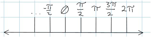
To get a numerical solution, the space we are working in (called the “domain”) is broken up into tiny pieces. This process is called discretizing. To see how this works, let’s first consider the number line as we know it. Since we’re dealing with sin and cos, let’s write the number line from 0 to  .
.

When we write the number line, we typically mark some values with the understanding that the intermediate values are there. I wrote  on one of the ticks, but we know that
  exists in there as well.
If we discretize (break into little pieces) the number line from
exists in there as well.
If we discretize (break into little pieces) the number line from  to it would look like this

What’s the difference? Here there are blocks and everywhere in the block has the same value. Take the block labeled . There is no in there. Everywhere in that block, the value is the same. At the faces between the blocks we can interpolate a value. These are marked, in this picture, by writing the numbers (0,  , etc) over the face.
Clearly, this is an approximation. Think of the distance from one cell to another as dx. Remember from calculus that dx is an infinitesimally small increment. On our discretized number line, it is no longer infinitesimally small. This is one potential pitfall with numerical solutions: if the dx isn’t small enough the answer will have too much error. Think about trying to plot sin(x) on the number line in the picture. What would it look like? Is that a good approximation of the real behavior of sin(x)?
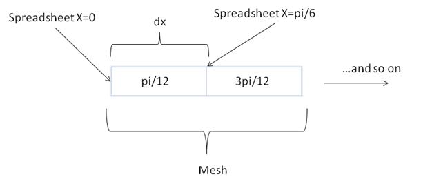
The equations are discretized as well. In our example, the value of cos(x) would be used at every point on our domain. This is simple to visualize using a spreadsheet.
Open your favorite spreadsheet program and create a discretized x-axis from to . To start with, we’ll break our number line down into cells of
, etc) over the face.
Clearly, this is an approximation. Think of the distance from one cell to another as dx. Remember from calculus that dx is an infinitesimally small increment. On our discretized number line, it is no longer infinitesimally small. This is one potential pitfall with numerical solutions: if the dx isn’t small enough the answer will have too much error. Think about trying to plot sin(x) on the number line in the picture. What would it look like? Is that a good approximation of the real behavior of sin(x)?
The equations are discretized as well. In our example, the value of cos(x) would be used at every point on our domain. This is simple to visualize using a spreadsheet.
Open your favorite spreadsheet program and create a discretized x-axis from to . To start with, we’ll break our number line down into cells of  . That will be the dx. Start with and add dx.
| dx | x |
| 0 | |
| 0.523599 | 0.523599 |
| 0.523599 | 1.047198 |
| 0.523599 | 1.570796 |
| 0.523599 | 2.094395 |
| 0.523599 | 2.617994 |
| 0.523599 | 3.141593 |
| 0.523599 | 3.665191 |
| 0.523599 | 4.18879 |
| 0.523599 | 4.712389 |
| 0.523599 | 5.235988 |
| 0.523599 | 5.759587 |
| 0.523599 | 6.283185 |
Now, calculate 
| dx | x | dy/dx |
| 0 | 1 | |
| 0.523599 | 0.523599 | 0.866025 |
| 0.523599 | 1.047198 | 0.5 |
| 0.523599 | 1.570796 | 6.13E-17 |
| 0.523599 | 2.094395 | -0.5 |
| 0.523599 | 2.617994 | -0.86603 |
| 0.523599 | 3.141593 | -1 |
| 0.523599 | 3.665191 | -0.86603 |
| 0.523599 | 4.18879 | -0.5 |
| 0.523599 | 4.712389 | -1.8E-16 |
| 0.523599 | 5.235988 | 0.5 |
| 0.523599 | 5.759587 | 0.866025 |
| 0.523599 | 6.283185 | 1 |
We’re now ready to numerically solve the equation. We know what the slope is – it’s dy/dx. So
should give us our

 . Remember how you generated your
  values? You started at the first value, , and added dx. We’ll do the same thing again. Start from the first y value. But what is that? We know that from the boundary condition. The boundary condition was when . So we start from . Just go down the y column and add dy to the previous y. If the cell that says “dx” is A1, input D3=C3*A3+D2, D4=C4*A4+D3, etc.
| dx | x | dy/dx | y| |
| 0 | 1 | 0 | |
| 0.523599 | 0.523599 | 0.866025 | 0.45345 |
| 0.523599 | 1.047198 | 0.5 | 0.715249 |
| 0.523599 | 1.570796 | 6.13E-17 | 0.715249 |
| 0.523599 | 2.094395 | -0.5 | 0.45345 |
| 0.523599 | 2.617994 | -0.86603 | 0 |
| 0.523599 | 3.141593 | -1 | -0.5236 |
| 0.523599 | 3.665191 | -0.86603 | -0.97705 |
| 0.523599 | 4.18879 | -0.5 | -1.23885 |
| 0.523599 | 4.712389 | -1.8E-16 | -1.23885 |
| 0.523599 | 5.235988 | 0.5 | -0.97705 |
| 0.523599 | 5.759587 | 0.866025 | -0.5236 |
| 0.523599 | 6.283185 | 1 | 0 |
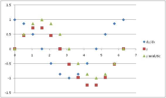
Excellent. Let’s plot our answer so we can look at it. Also, since we know the answer from the analytic solution, let’s plot that as well.

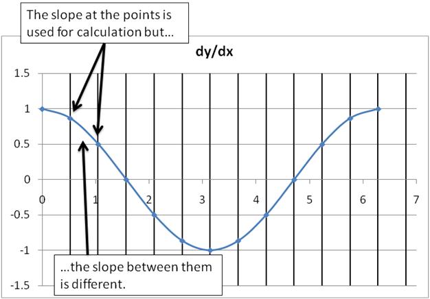
Hmm. Our solution doesn’t match the analytic solution so well (and we know the analytic solution is correct). What happened? Let’s examine some of the approximations we made. One of them was which value of dy/dx we used. The dx was constant, but in reality the dy is changing across our cells. Since we have discretized our space we lost this distinction.

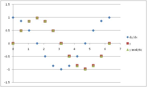
Really we should have used the value of dy at the face between the cells, not the value inside the cell. In this instance, since we know the answer we could cheat and just calculate the correct value. But in general we won’t have an analytic solution so we have to be more clever. We have to interpolate. Mathematicians and computer scientists have spent a lot of time thinking about how to interpolate values. For now, let’s just use a linear average of the values in the two cells while keeping in mind that there are many other ways to do it. For the harder problems, we’ll use software that takes care of this for us.
| dx | x | dy/dx | y |
| 0 | 1 | 0 | |
| 0.523599 | 0.523599 | 0.866025 | 0.488524 |
| 0.523599 | 1.047198 | 0.5 | 0.846149 |
| 0.523599 | 1.570796 | 6.13E-17 | 0.977049 |
| 0.523599 | 2.094395 | -0.5 | 0.846149 |
| 0.523599 | 2.617994 | -0.86603 | 0.488524 |
| 0.523599 | 3.141593 | -1 | 0 |
| 0.523599 | 3.665191 | -0.86603 | -0.48852 |
| 0.523599 | 4.18879 | -0.5 | -0.84615 |
| 0.523599 | 4.712389 | -1.8E-16 | -0.97705 |
| 0.523599 | 5.235988 | 0.5 | -0.84615 |
| 0.523599 | 5.759587 | 0.866025 | -0.48852 |
| 0.523599 | 6.283185 | 1 | -4.4E-16 |

That solution matches the analytic solution much better, doesn’t it?
Beginning with FiPy
Now, we’ll do the same exercise in FiPy. Start up a fresh window in your favorite Python editor. If you don't already have FiPy this is a good time to get it.
The easiest way to start using FiPy is to download the Matforge/FiPy live CD. Think of it as a fan mash-up of Ubuntu 9.10 and FiPy. It's designed to help you "jump start" using FiPy without needing to install FiPy and all of its dependencies. To use the live CD, download and burn the ISO image into a CD, and reboot your computer from the CD. The ISO image can also be used in a virtualization environment (e.g. VirtualBox?, VMWare, Parallels, KVM, Qemu, etc.) without needing to reboot the computer.
If you are a do-it-yourselfer, or you don't want to have to boot into another operating system to use FiPy you can install it. The developers of FiPy have created an installation guide for Windows, Mac, and Unix-based systems. Quick warning for Windows users: as of FiPy 2.1, you should install Python 2.5 (not 2.6) because one package that FiPy depends on (Pysparse) doesn't play well with Python 2.6.
Ready to roll? Good.
We’ll follow the same steps as when we solved the problem with the spreadsheet. Just like you had to open your spreadsheet program, you also have to “open” FiPy. This is done with the command
from fipy import *
Now, all the fipy commands are available to us.
Next, we discretize our domain. Fortunately, FiPy has built in functions that handle the messy stuff for us. We just have to tell it what we want. Let’s define the same dx. This is simple.
dx = pi/6.
We also have to define a number of points, nx.
nx=12.
That’s all the information it takes to create a discretized domain. We create the domain with the command
mesh=Grid1D(dx=dx, nx=nx)
Our domain information is stored in the variable called “mesh”. You can imagine the mesh like your blank spreadsheet. Since this is a 1-dimensional mesh, we have told the program that we will only be defining variables that use a single column of this spreadsheet at a time. . The mesh defines the domain we are working in. But we can’t store any information in the mesh. In just a bit we will define some variables (dy/dx) and tell them to use the mesh we have created. Defining the variables is just like filling their names in at the top of the spreadsheet and putting in their values. It’s important to check your work often to make sure you’re getting what you expect. A good check to see if your mesh is defined properly is
x = mesh.getCellCenters()[0]
print x
This assigns the value of every cell center to the variable x, and prints the value of x to the screen so we can see what it is. The output should be
[ 0.26179939 0.78539816 1.30899694 1.83259571 2.35619449 2.87979327
3.40339204 3.92699082 4.45058959 4.97418837 5.49778714 6.02138592]
These aren’t the same values we had for x in our spreadsheet. What happened? The difference is subtle, but important to keep in mind when doing numerical computing. When we defined x in our spreadsheet we were keeping track of the location of the cell edge. Remember, our domain is defined from 0 to , and our spreadsheet has both of those values. We’ve defined the same domain in fipy, but it keeps track of the cell centers. If you add pi/12 (that’s dx/2) to each of these values, you get the same numbers in our spreadsheet.

This distinction is not just academic. Fipy differentiates between variables defined at cell centers (called cell variables) from those defined at cell faces (called face variables). You already know why this is an important distinction to make. Remember when you made plot \label{fig:y_rightedgeslope}? The errors in that solution crept in because we weren’t careful which variables should be defined at the center, and which at the faces. Fipy is very particular about these things, and won’t let you add cell and face variables together. But we’ll deal with that when we come to it. Next we’ll define our variable. Just like in our spreadsheet we need to input what we know about dy/dx. We’ll define dy_dx as one of the cell variables we were just talking about. The only thing we need to tell fipy to make a cell variable is the mesh we are using. It’s good practice to give the cell variable a name also.
dy_dx = CellVariable(mesh=mesh, name='dy/dx')
dy_dx.setValue(cos(x))
We don’t strictly need to, but it’s much cleaner if we define dy as a separate variable.
dy = CellVariable(mesh=mesh, name='dy')
dy.setValue(dy_dx*dx)
Again, just like our spreadsheet, we’ll define y. But we’ll make y a face variable like it should be.
y= FaceVariable(mesh=mesh, value=0)
We included the “value=0” in the definition so that all the values in y start at 0. At the left edge, this is consistent with our boundary condition. But what about all those other values? We need to calculate them. In the future, we’ll let fipy do all the heavy lifting in solving these equations but this one we can do ourselves (especially since we’ve already written the algorithm in the spreadsheet). We’ll need to create an iterative solution since each value of y depends on the one before it. That sounds like a good job for a “for” loop. We also need some way to keep track of how many times we’ve run through the loop. One easy way to do this is to define an “index” counter and just iterate it each time through. With all that bookkeeping in place, all we have to do is apply the same algorithm we’ve already used.
index=0
for value in dy:
    index+=1
    y[index] = y[index-1]+value
    print y[index]
Take a second to convince yourself that this code does the same thing the spreadsheet does. Experienced python users will notice that we can operate on the CellVariable using [index] similar to a list. (Be careful. There are lots of commands that lists have that a CellVariable doesn't, and vice versa).
Using FiPy to Solve Differential Equations
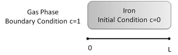
Now that we’ve seen all the steps to doing a simple numerical solution we’re going to learn to use some of the more powerful features of FiPy. These features will do a lot of what we just did for us, behind the scenes, so we don’t have to worry about it. So that we have something concrete to talk about, let’s solve one particular problem about the carburization of steel. Let’s say we have a sample of pure iron (0% carbon initially) and we flow a carbon containing gas (such as methane or carbon dioxide) over the sample. The flowing gas creates a constant concentration of carbon ( c=1) at the surface of the iron, which will diffuse into the bulk of the sample over time. The question is, what does the concentration profile (that’s a graph of C vs. Distance) look like at a given time t? You can assume a constant diffusivity, that the sample is infinitely thick, and that a one-dimensional answer is alright. You can also assume that the concentration in the gas phase is always c=1 and that we are only interested in the concentration of carbon in the iron.
Before we get to coding, it’s a good idea to ask ourselves a few questions. The answers to these questions will be the outline of the program. That way, in the future, when you have a different more difficult problem to solve you can ask yourself the same questions and come up with your own program. First question: what do we want to know? This is given in the problem. We want to know the concentration profile at a time t. This concentration profile will be given by an equation. That begs the second question. Second question: what is the equation? It’s the well known diffusion equation that you learned in your kinetics class:
We can solve that equation, but we need to know some boundary conditions first. Third question: what are the boundary conditions? We are going to need a boundary condition for the left and right edge of the domain. We can pull these out of the problem statement. We’re told that the concentration at the left edge (where the gas hits the sample) is c=1. But what about the right edge? This is a little more subtle. We’re told that the sample is effectively infinitely thick. That means that, in the time we’re willing to sit around and wait for this experiment to end, the carbon will never be able to diffuse all the way to the right edge. We also don’t want to discretize an infinite domain: that would be impossible! What we can do it make the right boundary condition c=0. This simulates the effect of having any carbon that hits the right edge of our domain continuing on its way through the infinite sample. Now that we know what the boundary conditions are, we need some way to start the problem. That’s called an initial condition. Fourth question: what is the initial condition? This one is easy. We’re told that the sample is pure iron at the beginning. So our initial condition is c=0 everywhere in the domain. What is the domain in the problem? That is the fifth question. The boundary conditions we’ve laid out say that the domain is the semi-infinite iron bar. The left edge (at
 ) touches the gas and the right edge (at
  ) simulates an infinite bar. Let’s do a quick sketch of what our system looks like.

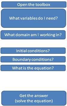
That’s all the material science questions we need to answer to solve this problem. The only thing left is to figure out what all our variables are. Sixth question: what variables do I need? Try to come up with the list on your own before reading the next paragraph. The problem talks about a diffusivity, so we’ll need that. We’ll also need a total length of the domain. What else are we missing? Think back to the problem we did about numerically integrating cos(x). In that case we needed a dx and also a number of points along the domain, nx. And just like we discretized space in that problem, we need to discretize time in this one (since we’re solving for dc/dt). Recap of the Variables:
- L --> length of domain
- D --> diffusivity
- nx --> number of discretized cells along x-axis
- dx --> how large each discretized cell is
- t --> how long we will run the simulation for. Said another way, the number of discretized time steps.
- timestepDuration --> how much time each time step represents.
The final question we have to ask is “how are we going to do all this?” FiPy has the tools we need, but we need to “open the toolbox.” The whole process is recapped below. We’re going to code up the answers to these questions in reverse order, so that’s how they’re listed below.

Look at all the work we’ve had to do before we even start programming. Start with a new, blank python file. Once we’ve built this program together you’ll see what goes into them and you’ll be able to do it yourself by answering the same series of questions. We’ll go through it together this first time so you can learn the syntax. Python, like many other languages, allows you to reuse code by “importing” it into the current program. This command is done with
from fipy import *
just like in the previous example. Now all the FiPy commands are available to us. Next, we need to define all our variables.
L = 1.
nx = 50.
dx = L / nx
timeStepDuration = 0.001
steps = 100
D = 0.5
It is easier to work in unitless space and time so let’s not worry about seconds or meters at this point. Consider this an abstract problem. An exercise at the end lets you apply units to this example. One thing to notice is that dx is defined in terms of L and nx. We could have just as easily defined dx and nx, in which case L would be nx*dx. Those three terms are all related. Do you see why? Next, we answer what domain we’re working in. The problem told us to work in one-dimension so that’s what we’ll do. Remembering that FiPy variables are built on grids, let’s make one of those and build our concentration variable on it.
mesh = Grid1D(dx = dx, nx = nx)
c = CellVariable(name = "concentration", mesh = mesh)
Next question: what are the initial conditions? Here, we just assign the initial values to c.
c.setValue(0.0)
This is a bit of a “gotcha” with the FiPy syntax. What if you had said
c=0
instead? The variable “c” would no longer be a cell variable, built on the FiPy mesh! It would instead be a simple integer value of zero. That’s because you assigned c to the value of zero. Remember to use the FiPy command .setValue to fill in the values for the CellVariable. Moving right along to the boundary conditions. Now we can really use some of the power of FiPy. Because boundary conditions are necessary to solve any differential equations, FiPy has a built-in way to handle boundary conditions.
boundaryConditions=(FixedValue(mesh.getFacesLeft(),1.0),
                   FixedValue(mesh.getFacesRight(),0.0))
Fittingly, if you wanted fixed flux boundary conditions, you could have said FixedFlux? instead of FixedValue?.
Next, let’s code the equation. This will be much easier using FiPy’s built-in tools than it was to do earlier. The syntax is a little tricky, but you can do it once you get the hang of it. FiPy has names for different terms. For any variable V if you have a term that looks like

We call that a transient term. If you have a term that looks like
It’s called a diffusion term. Easy enough to remember for us, but that this is true even if the process we’re modeling isn’t diffusion. Any

 term is referred to as a diffusion term.
Those are all the terms we need for now, we’re ready to declare our equation
term is referred to as a diffusion term.
Those are all the terms we need for now, we’re ready to declare our equation
eqn1 = TransientTerm() == ImplicitDiffusionTerm(D)
A couple notes about the syntax. We’re making a new variable called eqn1 and assigning it to have the value of everything to the right of the  sign. In the equation itself, we use the double equals
  . We also have to say "TransientTerm?()" instead of "TransientTerm?" because we are calling a built-in FiPy function. Finally, note that we didn’t need to tell FiPy that this equation is for the concentration c. We’ll do that when we solve it. Right now, this term eqn1 is just the generic form of any diffusion equation.
The problem is officially all set up. The only thing left is to solve the equation and get our answer.
. We also have to say "TransientTerm?()" instead of "TransientTerm?" because we are calling a built-in FiPy function. Finally, note that we didn’t need to tell FiPy that this equation is for the concentration c. We’ll do that when we solve it. Right now, this term eqn1 is just the generic form of any diffusion equation.
The problem is officially all set up. The only thing left is to solve the equation and get our answer.
for step in range(t):
        eqn1.solve(c, boundaryConditions = boundaryConditions, dt = timeStepDuration)
TSVViewer(vars=(c)).plot(filename="output.txt")
The loop iterates over all our time t. At each time we solve the equation, which is just as easy as using the “solve” command (if only everything were that easy). Notice that in the solve command, we finally tell FiPy what variable to use. We also have to tell it about the boundary conditions, and how long the timestep is. At the end of the loop we save the output text to a file. We could have also printed a graph to the screen.
Take a little time to go back over the code. Can you follow the logic of each step? Try these additional problems to test your understanding. If you'd like you can also download the example code.
Additional Problems
- Alter the script to show the concentration profiles at many different times.
- Redo the problem using realistic values with units.
- FiPy variables can store units. For example, you could declare dx=Variable(“3 cm”). Read the FiPy documentation about using these units and redo part (2) with the built-in unit capability.
- What if the sample were not infinitely thick but instead only 3 cm thick. How would the problem change?
- What if D(c) instead of a constant?
- What if D(x) instead of a constant?
Attachments (8)
- numberline.jpg (11.7 KB) - added by gathrw 5 years ago.
- plot_numeric_analytic_cos.jpg (17.3 KB) - added by gathrw 5 years ago.
- plot_numeric_analytic_cos_corrected.jpg (16.8 KB) - added by gathrw 5 years ago.
- slope_varies_between_cells.jpg (36.6 KB) - added by gathrw 5 years ago.
- cell_face_explaination.jpg (11.0 KB) - added by gathrw 5 years ago.
- sketch_of_domain.jpg (11.9 KB) - added by gathrw 5 years ago.
- questions_for_code.jpg (15.2 KB) - added by gathrw 5 years ago.
- discretizednumberline.jpg (11.2 KB) - added by gathrw 5 years ago.
Download all attachments as: .zip