

If you’ve never coded a finite element solver before — or if you know a few Python functions but have no idea where to begin — this is your roadmap.
Here’s exactly how top computational mechanics programs (Stanford, ETH Zurich, TUM) structure the journey from “first Python script” to “I’ve written my own FEM solver,” and what you should actually build at each stage.
Skip the guesswork. Follow the ladder.
TL;DR — What You Need to Know
The path in 6 steps:
- Build the three pillars first: applied mathematics, continuum mechanics, and computer science — all three are non-negotiable in computational mechanics.
- Start with a 1D spring element. That’s it. One element. One stiffness matrix. Nothing else matters until you can do this yourself.
- Progress through 1D → 2D → 3D: 1D springs, 2D meshes (triangles, quads), then 3D solids (tetrahedra, hexahedra). This is the proven progressive coding ladder.
- Learn software engineering in parallel: Git, testing, profiling, and modular code. Stanford teaches this before computational mechanics, not after.
- Use Python for learning, then graduated compiled languages: Python (NumPy, SciPy) is the right educational stack. Eventually learn C++ or Fortran for production-scale simulations.
- Build your own FE code before trusting commercial software: The Warwick study found 85% of students who wrote their own FE codes understood the material better than those who only used commercial tools.
The fastest way to start? Open a Jupyter notebook, write a 1D spring element solver, and stop looking at the menu bars in Abaqus.
The Three Pillars of Computational Mechanics
Computational mechanics lives at the intersection of three disciplines. If you’re only strong in one, you’ll hit walls — fast.
Applied mathematics gives you the language: linear algebra (matrix assembly, eigenvalue problems), calculus (gradients, integrals, PDEs), numerical analysis (stability, convergence, error estimation).
Continuum mechanics gives you the physics: stress-strain relations, equilibrium equations, boundary conditions, constitutive models.
Computer science gives you the tools: data structures, algorithms, memory management, parallelization, testing, profiling.
The AI Overview curriculum comparison from TUM COMMAS maps directly onto these pillars — Mathematics → Mechanics → Computation → Application — and it’s not coincidental. Programs that don’t teach all three in parallel produce students who can derive equations but can’t code them, or can code but don’t understand the physics.
If you’re starting from zero, the order matters. Here’s what I recommend:
- Start with math (linear algebra, calculus, introductory numerical methods) alongside basic Python programming.
- Simultaneously, begin reading continuum mechanics fundamentals — stress, strain, equilibrium.
- Layer in computer science early: Git, testing, and debugging patterns. Don’t wait until year three to care about version control.
The modeling pipeline from equations to simulation runs through all three pillars simultaneously. If you’re new to the full workflow, reading the From Equations to Simulations guide gives you the big-picture context before diving into the step-by-step ladder below.
The 1D → 2D → 3D Progressive Coding Ladder
This is the single most important framework in this article. Every computational mechanics student follows this progression, whether their program is explicit about it or not.
Phase 1: 1D — Springs and Bars (The Foundation)
What you’re learning: stiffness matrix assembly, nodal forces, boundary conditions, global coordinate mapping, elementary assembly.
What you build: a Python function that takes 1D spring elements, assembles a global stiffness matrix, applies boundary conditions, and solves F = Kx.
Concrete milestones:
- Solve a 5-spring series system with fixed end
- Add a node with prescribed displacement
- Map element coordinates to global coordinates
- Write a unit test that verifies force equilibrium
- Plot displacement vs position
Why this matters: If you can’t assemble a stiffness matrix by hand and write it in Python in an afternoon, you’re not ready for 2D. This is the moment where “FEM” stops being a buzzword and starts being a procedure you can execute.
Where to start: Read the What Is Scientific Simulation and Why It Matters article to understand the simulation ecosystem before you start coding. Then try this FiPy example to see how structured Python code handles discretization — even though it’s a diffusion problem, the discretization patterns transfer directly to FEM.
Phase 2: 2D — Meshes, Continua, and Reality (The Real Work)
What you’re learning: mesh generation (CST triangles, quadrilaterals), shape functions, numerical integration (Gauss quadrature), assembly of sparse matrices, solving larger systems.
What you build: a 2D elastic solver with mesh generation, shape function evaluation, and sparse matrix assembly.
Concrete milestones:
- Generate a triangular mesh for a square domain
- Implement CST (Constant Strain Triangle) shape functions
- Assemble a 2D elasticity stiffness matrix
- Apply plane stress vs. plane strain conditions
- Solve with SciPy’s sparse solver (scipy.sparse.linalg)
- Visualize deformed mesh with matplotlib
Why this matters: 2D is where FEM becomes actual engineering. You’re now dealing with meshes, shape functions, and the sparse matrix patterns that dominate real-world solvers. This is also where students typically encounter their first convergence studies.
The mesh quality lesson: Don’t skip convergence studies at this stage. This guide on mesh quality and convergence studies explains how to prove your solution is converging — not just guessing.
Phase 3: 3D — Solids, Continua, and Production Reality (The Capstone)
What you’re learning: 3D tetrahedral and hexahedral elements, solid mechanics (Lame’s parameters, Poisson’s ratio), adaptive mesh refinement, parallel assembly, performance bottlenecks.
What you build: a full 3D FEM solver with visualization, convergence verification, and performance profiling.
Concrete milestones:
- Generate tetrahedral mesh for a 3D domain
- Implement linear tetrahedron shape functions
- Assemble 3D elasticity stiffness matrix
- Profile your code (find bottlenecks)
- Add adaptive mesh refinement
- Compare against benchmark solution
Why this matters: 3D is where computational mechanics becomes production-grade. This is the capstone before graduate-level specialization. If you can build a working 3D FEM solver from scratch, you’re at the level of a junior simulation engineer.
Software Engineering Literacy — The Missing Parallel Track
Here’s what almost no undergraduate program does well: teaching software engineering alongside computational mechanics. Stanford’s CME 211 (Python/C++ for scientists and engineers) is the exception — and it’s exactly why Stanford graduates write better simulation code than most.
Why software engineering matters in simulation:
Your FEM code is not a homework assignment. It’s a research tool. It will run for hours or days. It will be shared with collaborators. It will be revisited months later. If your code can’t be versioned, tested, and profiled, you don’t have a research tool — you have a notebook with temporary scripts.
The software engineering checklist for students:
| Skill | When to learn it | Why it matters |
|---|---|---|
| Git + version control | Day 1 | Track every change; collaborate with peers |
| pytest + unit testing | Phase 1 (1D) | Verify your stiffness matrix assembles correctly |
| Debugging (print → profiler) | Phase 1-2 | Find memory leaks, incorrect indices, numerical errors |
| NumPy + SciPy | Phase 1 | Core scientific computing stack |
| Performance profiling | Phase 2 (2D) | Find bottlenecks before they become blockers |
| Modular code design | Phase 2-3 | Separate mesh generation, assembly, solve, visualize |
| Documentation | Phase 3 (3D) | Explain what your code does; publishable |
You can read Version Control Patterns for Scientific Software for branching strategies that actually work in research contexts, and Python Testing Patterns for Scientific Code for testing strategies that go beyond basic pytest assertions.
What I’d choose: Start with Git on day one. Add pytest in Phase 1. Add profiling in Phase 2. This sequence lets you catch errors before they compound. Don’t wait. The sooner you treat your code like software, the less you’ll regret it in Phase 3.
When to Use Python vs C++ vs Julia
This is the single most common student question I hear: “What language should I use?” The answer depends on your stage.
| Stage | Recommended language | Why |
|---|---|---|
| Phase 1-2 (learning) | Python (NumPy, SciPy) | Fastest feedback loop, rich ecosystem, Jupyter notebooks |
| Phase 3 (capstone) | Python + Cython | Performance optimization without abandoning Python |
| Production simulation | C++ or Fortran | Compiled, parallelizable, production-ready |
| ML surrogates / PINNs | Python (PyTorch, TensorFlow) | ML libraries are Python-first |
Python for learning — no debate. The scientific Python ecosystem (SciPy, NumPy, SymPy) gives you linear algebra, numerical integration, symbolic math, and plotting in one coherent stack. You cannot match this productivity in C++.
C++/Fortran for production — inevitable. Once your simulations are large enough that Python’s overhead matters (and they will be), you’ll need compiled code. C++ with Eigen or Armadillo, or Fortran with modern syntax, are the production standards.
Julia for the curious. Julia is gaining traction in computational mechanics (especially for PDE solvers via DifferentialEquations.jl). It’s faster than Python and more accessible than C++, but it’s not yet the standard for student education.
My recommendation: Learn Python thoroughly. Master NumPy, SciPy, and matplotlib. Then learn C++ (or Fortran) in parallel during Phase 2. By Phase 3, you’ll be ready to port performance-critical parts of your solver to compiled code. This is the progression Stanford’s CME 211→212 sequence effectively models.
Benchmarking Against Top Programs
What do the best computational mechanics programs actually look like? Here’s a comparison of four institutional benchmarks.
| Program | Duration | Structure | Key Features |
|---|---|---|---|
| TUM COMMAS | Master’s (4 semesters, 120 ECTS) | 4-phase progression | 120 ECTS total, foundations → electives → thesis, summer school with top researchers |
| Stanford CME | Graduate courses | Prerequisite → core → capstone | CME 211 (software engineering) → CME 232 (computational mechanics), CME 212 intermediate |
| ETH Zurich CSE | Bachelor’s (3 years, 180 credits) | Year 1-3 progression | Year 1: unified math/physics/CS, Year 2: natural sciences + engineering, Year 3: specialization + HPC |
| MIT OCW | Undergraduate | Course-by-course | Open courseware, no formal structured degree, but excellent individual modules |
ETH Zurich’s BSc CSE is the closest undergraduate equivalent to a “computational mechanics” learning path. Unlike most programs that treat computational science as a supporting course, ETH treats it as a first-class discipline with its own degree program. Year 1 forces unified math/physics/CS. Year 2 deepens in natural sciences. Year 3 specializes. This is the rare program that actually structures the full progression.
If you’re at a program without a structured path (which is most of them), use these benchmarks to evaluate your own curriculum. Where is it light? Where are you strong? Fill the gaps deliberately.
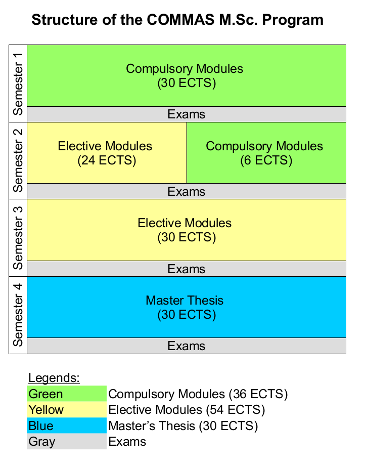
Curriculum structure from the COMMAS Summer School program at the University of Stuttgart — shows the phased progression from foundations to thesis.
What to Actually Build — A Student’s Project Roadmap
Theory is invisible without concrete projects. Here’s the progression I recommend, ordered by difficulty and educational value.
Level 1 — 1D Spring Element (2-4 hours)
- Write a function that assembles a global stiffness matrix from N spring elements
- Apply Dirichlet boundary conditions
- Solve with
numpy.linalg.solve - Plot displacement
- This is your first FEM code. Nothing before it matters until this works.
Level 2 — 2D Elasticity Solver (1-2 weeks)
- Generate a triangular mesh (or import one)
- Implement CST shape functions
- Assemble 2D elasticity stiffness matrix
- Solve with
scipy.sparse.linalg - Visualize deformed mesh
- This is the real engineering stage. This is where FEM becomes actual engineering.
Level 3 — 3D Solid Mechanics Solver (3-6 weeks)
- Generate tetrahedral mesh
- Implement linear tetrahedron shape functions
- Assemble 3D stiffness matrix
- Add adaptive mesh refinement
- Profile and optimize
- Compare against benchmark solution
Level 4 — Solver Comparison (advanced)
- Compare your solver against FEniCS or FiPy
- Benchmark accuracy, speed, memory
- Write a comparison report
- This teaches you to use open-source tools critically, not just as black boxes.
You can find starter code for some of these in the Student Project Ideas list — not as learning paths, but as concrete templates you can study and adapt.
Evidence: Why Hands-On Coding Beats Black-Box Training
Let me be direct about what the research shows: writing your own FE code beats learning commercial software menus every time.
The Warwick study (Khajehsaeid & Riazifar, 2023) surveyed students who built and tailored their own finite element codes — starting in 2D, extending to 3D — and compared them against students who only used commercial FE packages.
The result: 85% of students who wrote their own codes reported that it “helped understand how theory translates to problem-solving tools and FE software.” That’s not a small majority. That’s an overwhelming consensus.
Students who used only commercial software (Abaqus, ANSYS, COMSOL) could run simulations. They could click menus. But they couldn’t explain what their software was actually computing.
Students who wrote their own codes understood:
- What the stiffness matrix actually represents
- How boundary conditions modify the system
- Why numerical integration matters
- When to trust or distrust results
My recommendation: Start with your own 1D solver. Move to 2D. Then use FEniCS or FiPy as verification tools — not replacements. This is the progression the Warwick study validated.
If you’re confused about when to use FEM vs FVM vs FDM, start by reading this practical comparison. It explains the differences clearly before you start coding.
Your Next Steps — Where to Start Today
You don’t need to wait for a class. You don’t need permission. Here’s exactly what to do next:
- Install Python, NumPy, SciPy, and matplotlib. If you need help, this guide on the scientific Python ecosystem walks you through the full stack.
- Write a 1D spring element. Five springs. Fixed end. Solve. Plot. Nothing more.
- Commit it to Git. Day one. Track every change. Learn branching.
- Add a unit test. Verify force equilibrium. Prove your code works.
- Extend to 2D. CST triangles. Mesh generation. Sparse assembly.
- Profile. Optimize. Repeat. Find bottlenecks with this profiling guide.
The single most important step? Start with the 1D spring element. Stop looking at the menu bars in Abaqus. Build your own solver. That’s the difference between knowing FEM and understanding it.
Want to explore FiPy first? Start with the FiPy documentation and work through this diffusion example. It won’t teach you FEM directly, but it will teach you the Python patterns that transfer.
Related Guides
- From Equations to Simulations: The Modeling Pipeline — Big-picture context for the full simulation workflow
- When to Use FEM, FVM, or FDM — Practical comparison of discretization methods for beginners
- The Scientific Python Ecosystem — Tool stack overview for simulation
- Solving Diffusion Equations with FiPy — Concrete Python example to study
- Unit Testing for Scientific Code — Testing strategies that go beyond basic assertions
- Version Control Patterns for Scientific Software — Git branching strategies for research
- Scientific Computing Performance Profiling — Identifying and fixing bottlenecks
- Mesh Quality and Convergence Studies — How to prove your solution is converging
- GPU Acceleration for FiPy Simulations — Scaling up to GPU computing
- Choosing the Right Python PDE Solver — FiPy vs py-pde vs FEniCS comparison
- HPC Python Workflows — Scaling from laptop to supercomputer
This article maps the step-by-step progression from “first Python script” to “own FEM solver,” using institutional benchmarks from TUM COMMAS, Stanford CME, ETH Zurich CSE, and MIT OCW as structural guides. The 1D → 2D → 3D coding ladder is the single most important framework — follow it, and you’ll build real understanding, not just software familiarity.